
<p><strong>线性变换</strong></p> x’=Ax,其中A是矩阵,x’和x都是向量,这是一种原点不变,且原有的平行关系和倍数关系都不变的空间视角转换,它转换的是从不同空间视角来看x这个向量,x’和x其实是同一个向量,只不过所看的视角不同罢了。具体的内容可以参考线性代数整理(二) 中的线性变换。它是所有计算机图形学的基础。
仿射变换
仿射变换是在线性变换的基础上,原点可以发生变换。
x’=Ax+b,其中A是矩阵,x’、x、b都是向量。
仿射变换是单纯对图片进行平移、缩放、倾斜和旋转,而这几个操作都不会改变图片线之间的平行关系。如果用三维线性表达就是
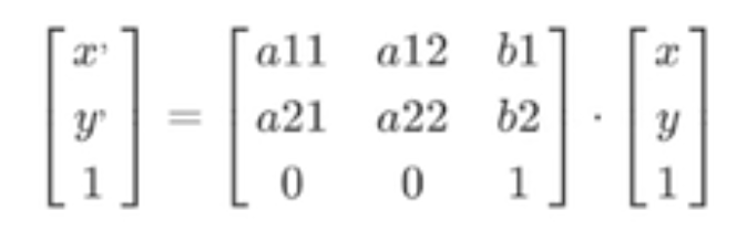
那么它又满足了线性变换的基本格式,具体实例可以参考OpenCV计算机视觉整理 中的图像的仿射变换。这里我们将不使用opencv内置方法,而使用numpy来重写第二个图形旋转实例,方便理解。
import numpy as np
import math
from PIL import Image
import cv2

def
affine_transform_numpy(image, transform_matrix):
    """


使用
numpy
实现仿射变换

    Args:

        image:
输入图像的
numpy
数组
 (H, W, C)

        transform_matrix: 2x3
的仿射变换矩阵

    Returns:


变换后的图像
numpy
数组
    """

    h, w, channels = image.shape

    #
创建输出图像

    output = np.zeros_like(image)

    #
计算变换矩阵的逆矩阵(用于反向映射)


#
将
2x3
矩阵扩展为完整的
3x3
矩阵,对应公式中的完整变换矩阵
:

    # [a11  a12  b1]

    # [a21  a22  b2]

    # [0    0    1 ]  <-
齐次坐标的底行

    full_matrix = np.vstack([transform_matrix, [0, 0, 1]])
    print("
完整的
3x3
变换矩阵
:")
    print(full_matrix)
    try:
        #
计算逆矩阵
 -
用于反向映射


#
正向映射
: [x', y'] = M * [x, y]  (
从原图到目标图
)

        #
反向映射
: [x, y] = M^(-1) * [x', y']  (
从目标图回到原图
)

        inv_matrix = np.linalg.inv(full_matrix)
        print("
逆变换矩阵
:")
        print(inv_matrix)
        inv_transform = inv_matrix[:2, :]  #
取前两行,得到
2x3
逆变换矩阵


print("
用于反向映射的
2x3
矩阵
:")
        print(inv_transform)
    except np.linalg.LinAlgError:
        print("
变换矩阵不可逆,返回原图像
")
        return image

    #
创建目标图像的坐标网格
 -
对应公式中的
 [x', y', 1]

    y_coords, x_coords = np.mgrid[0:h, 0:w]
    #
将坐标转换为齐次坐标形式
 [x', y', 1]
,每列是一个像素的坐标

    coords = np.stack([x_coords.ravel(), y_coords.ravel(), np.ones(x_coords.size)])
    print("
目标图像坐标矩阵形状
:", coords.shape)
    print("
前
5
个像素的齐次坐标
:
\n
", coords[:, :5])

    #
应用逆变换获取源图像坐标,跟原始公式不同,这里使用的是逆变换,
@
在
python
中是矩阵乘法


# [x, y, 1]^T = M^(-1) * [x', y', 1]^T

    source_coords = inv_transform @ coords
    source_x = source_coords[0].reshape(h, w)
    source_y = source_coords[1].reshape(h, w)

    #
双线性插值


for c in
range(channels):
        output[:, :, c] = bilinear_interpolation(image[:, :, c], source_x, source_y)

    return output.astype(np.uint8)

def
bilinear_interpolation(image, x_coords, y_coords):
    """


双线性插值

    Args:

        image:
单通道图像
 (H, W)

        x_coords: x
坐标数组
        y_coords: y
坐标数组

    Returns:


插值后的图像
    """

    h, w = image.shape
    output = np.zeros_like(x_coords)

    #
找到有效的坐标范围

    valid_mask = (x_coords >= 0) & (x_coords < w - 1) & (y_coords >= 0) & (y_coords < h - 1)

    #
获取有效坐标

    valid_x = x_coords[valid_mask]
    valid_y = y_coords[valid_mask]

    if
len(valid_x) == 0:
        return output

    #
计算整数和小数部分

    x0 = np.floor(valid_x).astype(int)
    y0 = np.floor(valid_y).astype(int)
    x1 = x0 + 1

    y1 = y0 + 1


#
确保坐标在有效范围内

    x1 = np.clip(x1, 0, w - 1)
    y1 = np.clip(y1, 0, h - 1)

    #
计算权重

    dx = valid_x - x0
    dy = valid_y - y0

    #
双线性插值


# I(x,y) = I(x0,y0)(1-dx)(1-dy) + I(x1,y0)dx(1-dy) + I(x0,y1)(1-dx)dy + I(x1,y1)dxdy

    interpolated = (image[y0, x0] * (1 - dx) * (1 - dy) +
                    image[y0, x1] * dx * (1 - dy) +
                    image[y1, x0] * (1 - dx) * dy +
                    image[y1, x1] * dx * dy)

    output[valid_mask] = interpolated

    return output

def
create_rotation_matrix(theta):
    """


创建旋转变换矩阵


    Args:

        theta:
旋转角度(弧度)


    Returns:

        2x3
的旋转矩阵
    """

    cos_theta = math.cos(theta)
    sin_theta = math.sin(theta)

    #
对应公式中的
2x3
变换矩阵
:

    # [a11  a12  b1]   [cos(θ)   sin(θ)  0]

    # [a21  a22  b2] = [-sin(θ)  cos(θ)  0]

    #
这是纯旋转矩阵,没有平移分量
 (b1=0, b2=0)

    rotation_matrix = np.array([
        [cos_theta, sin_theta, 0],      # [a11, a12, b1]

        [-sin_theta, cos_theta, 0]      # [a21, a22, b2]

    ], dtype=np.float32)

    return rotation_matrix

def
create_translation_matrix(tx, ty):
    """


创建平移变换矩阵

    Args:

        tx: x
方向平移量
        ty: y
方向平移量

    Returns:

        2x3
的平移矩阵
    """

    translation_matrix = np.array([
        [1, 0, tx],
        [0, 1, ty]
    ], dtype=np.float32)

    return translation_matrix

if __name__ == "__main__":
    try:
        #
使用
PIL
读取图像

        pil_image = Image.open("/Users/admin/Documents/111.jpeg")
        #
转换为
numpy
数组

        img = np.array(pil_image)

        if
len(img.shape) == 3:
            h, w, ch = img.shape
        else:
            #
如果是灰度图像,添加通道维度

            img = np.expand_dims(img, axis=2)
            h, w, ch = img.shape

        print(f"
图像尺寸
:
{h}
x
{w}
x
{ch}
")

        #
创建旋转变换矩阵(逆时针旋转
15
度)

        theta = math.pi / 12
# 15
度

        rotation_matrix = create_rotation_matrix(theta)

        #
可以组合多个变换,例如先旋转再平移


# translation_matrix = create_translation_matrix(100, 100)

        # combined_matrix = translation_matrix @ np.vstack([rotation_matrix, [0, 0, 1]])

        # transform_matrix = combined_matrix[:2, :]

        #
旋转矩阵是
2*2
的,这里没有平移,故变换矩阵只有旋转矩阵

        transform_matrix = rotation_matrix

        print("
变换矩阵
:")
        print(transform_matrix)

        #
应用仿射变换


print("
正在进行仿射变换
...")
        transformed_img = affine_transform_numpy(img, transform_matrix)

        #
转换图像格式用于
opencv
显示
 (RGB -> BGR)


if ch == 3:
            img_bgr = cv2.cvtColor(img, cv2.COLOR_RGB2BGR)
            transformed_img_bgr = cv2.cvtColor(transformed_img, cv2.COLOR_RGB2BGR)
        else:
            img_bgr = img
            transformed_img_bgr = transformed_img

        #
使用
opencv
显示图像

        cv2.namedWindow('Original Image', cv2.WINDOW_NORMAL)
        cv2.namedWindow('Transformed Image', cv2.WINDOW_NORMAL)

        cv2.imshow('Original Image', img_bgr)
        cv2.imshow('Transformed Image', transformed_img_bgr)

        print("
按任意键关闭窗口
...")
        cv2.waitKey(0)
        cv2.destroyAllWindows()

        #
保存变换后的图像

        output_pil = Image.fromarray(transformed_img)
        output_path = "/Users/admin/Documents/111_transformed.jpeg"

        output_pil.save(output_path)
        print(f"
变换后的图像已保存到
:
{output_path}
")

    except
FileNotFoundError:
        print("
错误
:
找不到图像文件
 /Users/admin/Documents/111.jpeg")
        print("
请确保图像文件存在,或修改文件路径
")
    except
Exception
as e:
        print(f"
处理图像时发生错误
:
{e}
")
这是反向映射的代码,对于完全满足公式的正向映射代码如下
import numpy as np
import math
from PIL import Image
import cv2

def
affine_transform_numpy(image, transform_matrix, fill_holes=True):
    """


使用
numpy
实现仿射变换(正向映射,优化版)

    Args:

        image:
输入图像的
numpy
数组
 (H, W, C)

        transform_matrix: 2x3
的仿射变换矩阵
        fill_holes:
是否填充空洞,默认
True

    Returns:


变换后的图像
numpy
数组
    """

    h, w, channels = image.shape

    #
创建输出图像

    output = np.zeros_like(image)

    #
正向映射:使用原始变换矩阵,完全按照数学公式


# [x', y'] = M * [x, y]  (
从原图到目标图
)


print("
正向映射变换矩阵
 (2x3):")
    print(transform_matrix)

    #
优化坐标计算:直接创建坐标矩阵


print("
创建坐标网格
...")
    y_indices, x_indices = np.mgrid[0:h, 0:w]

    #
创建齐次坐标矩阵
 (3, h*w)

    coords = np.vstack([
        x_indices.ravel(),
        y_indices.ravel(),
        np.ones(h * w, dtype=np.float32)
    ])

    print("
原图像坐标矩阵形状
:", coords.shape)
    print("
前
5
个像素的齐次坐标
:
\n
", coords[:, :5])

    #
应用正向变换获取目标图像坐标,完全按照原始公式,
@
在
python
中是矩阵乘法


# [x', y']^T = M * [x, y, 1]^T


print("
计算变换后坐标
...")
    target_coords = transform_matrix @ coords
    target_x = target_coords[0].reshape(h, w)
    target_y = target_coords[1].reshape(h, w)

    print("
变换后坐标范围
:")
    print(f"x': [
{np.min(target_x):
.2f
}
,
{np.max(target_x):
.2f
}
]")
    print(f"y': [
{np.min(target_y):
.2f
}
,
{np.max(target_y):
.2f
}
]")

    #
正向映射:使用向量化操作,大幅提升性能


print("
使用向量化操作进行正向映射
...")

    #
向量化处理:找到所有有效的目标坐标

    valid_mask = ((target_x >= 0) & (target_x < w) &
                  (target_y >= 0) & (target_y < h))

    #
获取有效的坐标

    valid_target_x = target_x[valid_mask]
    valid_target_y = target_y[valid_mask]

    #
四舍五入到整数坐标

    target_x_int = np.round(valid_target_x).astype(int)
    target_y_int = np.round(valid_target_y).astype(int)

    #
确保坐标在边界内(向量化
clip
操作)

    target_x_int = np.clip(target_x_int, 0, w - 1)
    target_y_int = np.clip(target_y_int, 0, h - 1)

    #
获取对应的原图像坐标

    y_coords_flat = np.repeat(np.arange(h), w)
    x_coords_flat = np.tile(np.arange(w), h)

    valid_y_orig = y_coords_flat[valid_mask.ravel()]
    valid_x_orig = x_coords_flat[valid_mask.ravel()]

    #
向量化复制像素值


if channels == 1:
        output[target_y_int, target_x_int] = image[valid_y_orig, valid_x_orig]
    else:
        for c in
range(channels):
            output[target_y_int, target_x_int, c] = image[valid_y_orig, valid_x_orig, c]

    #
可选的后处理:填补空洞


if fill_holes:
        output = fill_holes_simple(output)

    print(f"
变换完成!有效像素比例
:
{np.sum(output > 0) / output.size * 100
:
.2f
}
%")

    return output.astype(np.uint8)

def
fill_holes_simple(image):
    """


优化的空洞填充算法(向量化实现)

    使用邻域平均值填充空洞(像素值为
0
的位置)


    Args:

        image:
包含空洞的图像


    Returns:


填充后的图像
    """


if np.all(image != 0):
        return image  #
没有空洞,直接返回


print("
正在填充空洞
...")
    output = image.copy()
    h, w = image.shape[:2]

    #
使用卷积进行快速邻域填充


from scipy import ndimage

    if
len(image.shape) == 3:
        channels = image.shape[2]
        for c in
range(channels):
            channel = image[:, :, c]
            #
找到空洞位置

            holes = (channel == 0)

            if np.any(holes):
                #
使用均值滤波填充


#
创建权重矩阵(忽略
0
值)

                weights = (channel > 0).astype(float)

                #
计算加权平均

                kernel = np.ones((3, 3))
                sum_values = ndimage.convolve(channel.astype(float), kernel, mode='constant')
                sum_weights = ndimage.convolve(weights, kernel, mode='constant')

                #
避免除以
0

                valid_weights = sum_weights > 0

                filled_values = np.zeros_like(sum_values)
                filled_values[valid_weights] = sum_values[valid_weights] / sum_weights[valid_weights]

                #
只在空洞位置填充

                output[holes, c] = filled_values[holes]
    else:
        #
灰度图像

        holes = (image == 0)

        if np.any(holes):
            weights = (image > 0).astype(float)

            kernel = np.ones((3, 3))
            sum_values = ndimage.convolve(image.astype(float), kernel, mode='constant')
            sum_weights = ndimage.convolve(weights, kernel, mode='constant')

            valid_weights = sum_weights > 0

            filled_values = np.zeros_like(sum_values)
            filled_values[valid_weights] = sum_values[valid_weights] / sum_weights[valid_weights]

            output[holes] = filled_values[holes]

    return output

def
bilinear_interpolation(image, x_coords, y_coords):
    """


双线性插值

    Args:

        image:
单通道图像
 (H, W)

        x_coords: x
坐标数组
        y_coords: y
坐标数组

    Returns:


插值后的图像
    """

    h, w = image.shape
    output = np.zeros_like(x_coords)

    #
找到有效的坐标范围

    valid_mask = (x_coords >= 0) & (x_coords < w - 1) & (y_coords >= 0) & (y_coords < h - 1)

    #
获取有效坐标

    valid_x = x_coords[valid_mask]
    valid_y = y_coords[valid_mask]

    if
len(valid_x) == 0:
        return output

    #
计算整数和小数部分

    x0 = np.floor(valid_x).astype(int)
    y0 = np.floor(valid_y).astype(int)
    x1 = x0 + 1

    y1 = y0 + 1


#
确保坐标在有效范围内

    x1 = np.clip(x1, 0, w - 1)
    y1 = np.clip(y1, 0, h - 1)

    #
计算权重

    dx = valid_x - x0
    dy = valid_y - y0

    #
双线性插值


# I(x,y) = I(x0,y0)(1-dx)(1-dy) + I(x1,y0)dx(1-dy) + I(x0,y1)(1-dx)dy + I(x1,y1)dxdy

    interpolated = (image[y0, x0] * (1 - dx) * (1 - dy) +
                    image[y0, x1] * dx * (1 - dy) +
                    image[y1, x0] * (1 - dx) * dy +
                    image[y1, x1] * dx * dy)

    output[valid_mask] = interpolated

    return output

def
create_rotation_matrix(theta):
    """


创建旋转变换矩阵


    Args:

        theta:
旋转角度(弧度)


    Returns:

        2x3
的旋转矩阵
    """

    cos_theta = math.cos(theta)
    sin_theta = math.sin(theta)

    #
对应公式中的
2x3
变换矩阵
:

    # [a11  a12  b1]   [cos(θ)   sin(θ)  0]

    # [a21  a22  b2] = [-sin(θ)  cos(θ)  0]

    #
这是纯旋转矩阵,没有平移分量
 (b1=0, b2=0)

    rotation_matrix = np.array([
        [cos_theta, sin_theta, 0],      # [a11, a12, b1]

        [-sin_theta, cos_theta, 0]      # [a21, a22, b2]

    ], dtype=np.float32)

    return rotation_matrix

def
create_translation_matrix(tx, ty):
    """


创建平移变换矩阵

    Args:

        tx: x
方向平移量
        ty: y
方向平移量

    Returns:

        2x3
的平移矩阵
    """

    translation_matrix = np.array([
        [1, 0, tx],
        [0, 1, ty]
    ], dtype=np.float32)

    return translation_matrix

if __name__ == "__main__":
    try:
        #
使用
PIL
读取图像

        pil_image = Image.open("/Users/admin/Documents/111.jpeg")
        #
转换为
numpy
数组

        img = np.array(pil_image)

        if
len(img.shape) == 3:
            h, w, ch = img.shape
        else:
            #
如果是灰度图像,添加通道维度

            img = np.expand_dims(img, axis=2)
            h, w, ch = img.shape

        print(f"
图像尺寸
:
{h}
x
{w}
x
{ch}
")

                #
创建旋转变换矩阵(逆时针旋转
15
度)

        theta = math.pi / 12
# 15
度

        rotation_matrix = create_rotation_matrix(theta)

        #
可以组合多个变换,例如先旋转再平移


# translation_matrix = create_translation_matrix(100, 100)

        # combined_matrix = translation_matrix @ np.vstack([rotation_matrix, [0, 0, 1]])

        # transform_matrix = combined_matrix[:2, :]


        #
正向映射:直接使用
2x3
变换矩阵,按照数学公式
 [x', y'] = M * [x, y, 1]

        transform_matrix = rotation_matrix

        print("
变换矩阵
:")
        print(transform_matrix)

        #
应用仿射变换(正向映射)


print("
正在进行仿射变换(正向映射)
...")
        import time
        start_time = time.time()

        #
可以选择是否填充空洞(填充空洞会增加处理时间)

        fill_holes_option = True
#
改为
False
可以跳过空洞填充,提升性能

        transformed_img = affine_transform_numpy(img, transform_matrix, fill_holes=fill_holes_option)

        end_time = time.time()
        print(f"
变换耗时
:
{end_time - start_time:
.3f
}
秒
")

        #
转换图像格式用于
opencv
显示
 (RGB -> BGR)


if ch == 3:
            img_bgr = cv2.cvtColor(img, cv2.COLOR_RGB2BGR)
            transformed_img_bgr = cv2.cvtColor(transformed_img, cv2.COLOR_RGB2BGR)
        else:
            img_bgr = img
            transformed_img_bgr = transformed_img

        #
使用
opencv
显示图像

        cv2.namedWindow('Original Image', cv2.WINDOW_NORMAL)
        cv2.namedWindow('Transformed Image', cv2.WINDOW_NORMAL)

        cv2.imshow('Original Image', img_bgr)
        cv2.imshow('Transformed Image', transformed_img_bgr)

        print("
按任意键关闭窗口
...")
        cv2.waitKey(0)
        cv2.destroyAllWindows()

        #
保存变换后的图像

        output_pil = Image.fromarray(transformed_img)
        output_path = "/Users/admin/Documents/111_transformed.jpeg"

        output_pil.save(output_path)
        print(f"
变换后的图像已保存到
:
{output_path}
")

    except
FileNotFoundError:
        print("
错误
:
找不到图像文件
 /Users/admin/Documents/111.jpeg")
        print("
请确保图像文件存在,或修改文件路径
")
    except
Exception
as e:
        print(f"
处理图像时发生错误
:
{e}
")
透视变换
仿射变换是在二维空间中的旋转、平移和缩放,透视变换是在三维空间中的视角变化。相对于仿射,透视变换能保持”直线性”,原图像中的直线,经透视变换后仍为直线。
如果说仿射变换是对三维空间中某个平面的一些二维变化,透视变换就是对这个平面进行变换,并且利用视觉原理对图像进行一定处理(近大、远小)。
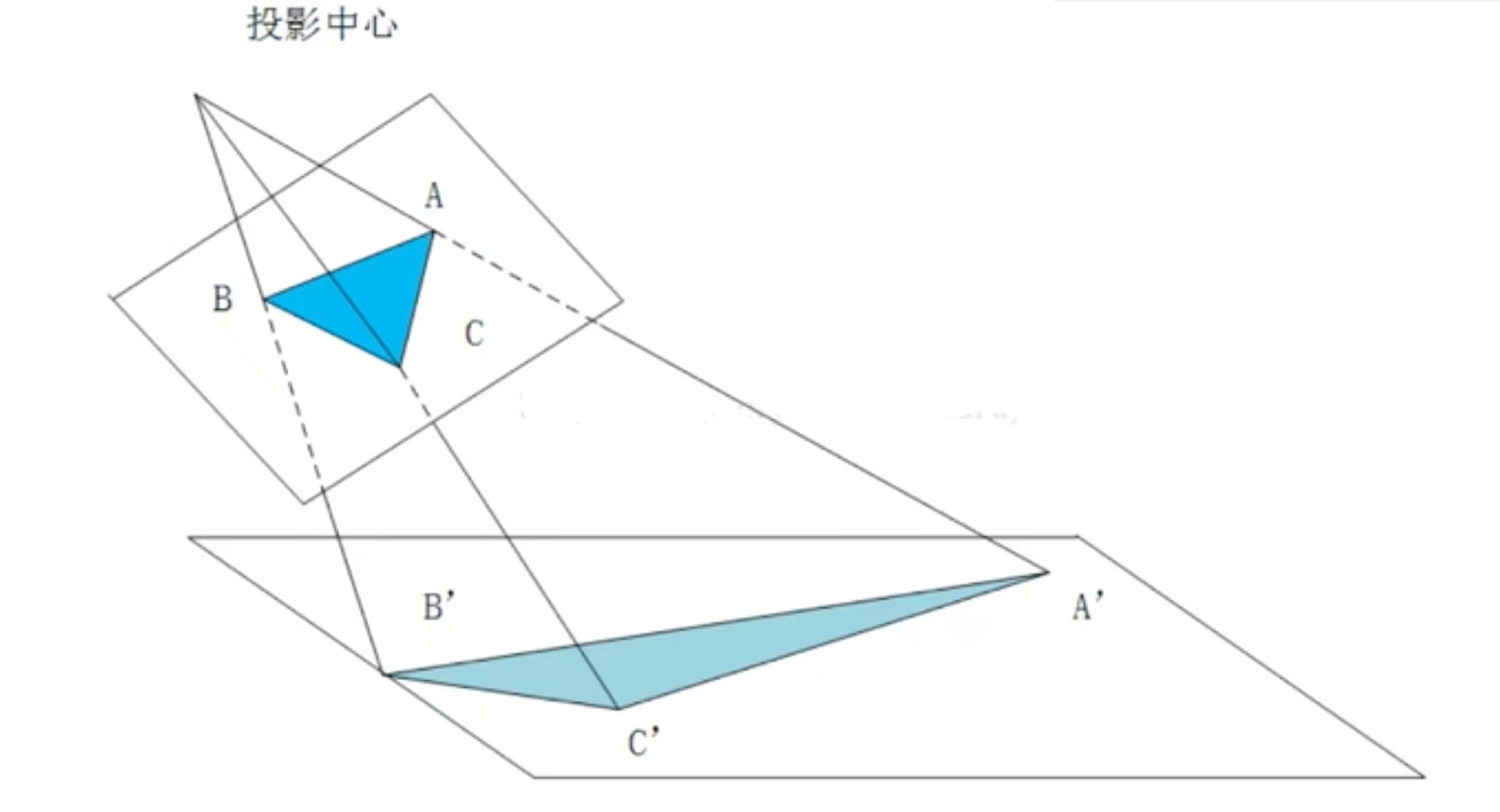
- 投影中心(Projection Center)
- 图中顶部标注的”投影中心”是透视变换的核心点
- 就像人的眼睛位置或相机镜头的光心
- 所有的投影线都从这个点发出
- 原始图形:三角形ABC
- 深蓝色三角形ABC是原始图形
- 位于较近的投影平面上
- 各个顶点坐标为A、B、C
- 变换后图形:三角形A’B’C’
- 浅蓝色三角形A’B’C’是透视变换的结果
- 位于较远的投影平面上
- 各个顶点坐标为A’、B’、C’
- 第一步:建立投影射线,从投影中心分别向原图形的每个顶点画射线:
- 投影中心 → A点:形成射线PA
- 投影中心 → B点:形成射线PB
- 投影中心 → C点:形成射线PC
- 第二步:确定目标投影平面,设定一个新的投影平面(图中下方的平面),这个平面通常:
- 平行于原平面,但距离投影中心更远
- 或者以某个角度倾斜
- 第三步:计算交点坐标,每条投影射线与目标平面的交点就是变换后的坐标:
- 射线PA与目标平面交于A’
- 射线PB与目标平面交于B’
- 射线PC与目标平面交于C’
- 第四步:形成变换结果
- 连接新的顶点A’、B’、C’,形成变换后的三角形
- 注意:形状发生了显著变化,不再是相似变换
- 非线性变换
- 直线仍保持直线(除了通过投影中心的直线)
- 角度不保持不变**
- 长度比例不保持不变**
- 面积比例不保持不变**
- 齐次坐标表示,透视变换使用齐次坐标:
- [x’] [h11 h12 h13] [x]
- [y’] = [h21 h22 h23] [y]
- [w’] [h31 h32 h33] [w]
- 最终坐标:x_final = x’/w’, y_final = y’/w’
- 近大远小效应
- 从图中可以看出,离投影中心近的物体(ABC)看起来较大
- 离投影中心远的物体(A’B’C’)看起来较小
- 这正是透视效果的本质
齐次坐标系与笛卡尔坐标系
我们说透视变换是非线性变换,但是从上面的公式来看,在齐次坐标系中它满足线性变换的基本格式,但最终我们需要转换回笛卡尔坐标。
齐次坐标系
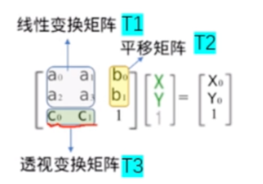
我们知道线性变换x’=Ax无法改变原点,即无法发生位移。但仿射变换x’=Ax+b可以,为什么我们要将这一加法操作转变为直接的矩阵乘法操作呢?
我们将平移值\([b_1 b_2]^T\),即向量b放在矩阵的右上角达到了相同的结果
- \(x’=a_{11}x+a_{12}y+b_1\)
- \(y’=a_{21}x+a_{22}y+b_2\)
- 1=1
这里的1=1很重要,我们知道对于平面上的运算,二维就够了,可为什么要用到三维坐标呢?这里就需要引入齐次坐标的概念。
齐次坐标是一种用n+1维来表示n维点的方法。简单来说,就是用额外的维度来表示点的”权重”或”深度”。它的好处就是可以使用矩阵乘法。
对于计算机来说,如果只使用二维的加法运算,对于一个图形有大量的点,计算耗时耗力,而矩阵乘法对于GPU来说,只需要一步完成。
而齐次坐标由\([x\ y\ 1]^T\)变成\([x\ y\ 0]^T\)时,其实就是没有平移的线性变换,原点不变。但其实齐次坐标为0时又表示平面内的无穷远点,我们知道只有二维坐标\([x\ y]^T\)时,无论x,y取何值,都无法表达∞这个概念,而\([x\ y\ 0]^T\)的齐次坐标则表达为无穷远点,它只表达方向。那既不是1又不是0时会怎样呢?如\([x\ y\ w]^T\),可以看作是3D空间中从原点出发的射线。在这种情况下,规则是要将恢复的的向量的每个分量除以齐次坐标w,以使齐次值回到1
\([\frac {x}{w}\ \frac {y}{w}\ 1]^T\)
那么这里的\(\frac {x}{w}\)和\(\frac {y}{w}\)就是笛卡尔坐标系中的坐标。齐次坐标w表示一个归一化的深度值,该值越大,投影后的物体越小;该值越小,投影后的物体越大。这里我们用透镜成像来理解就会更简单。
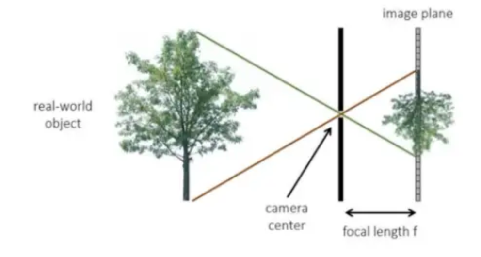
上图中,投影中心就是透镜的中心点,它到真实物体树的垂直距离为Z,它到后方投影平面的距离为焦距f,则\(w=\frac {Z}{f}\),在f固定不变的情况下,Z越大,w越大,在成像平面中,树的像就越小(这里需要注意的是树不是等比例放大的,它在任何位置都是同样大小的,越远的树的上下两端与原点的夹角就会越小,成像也会越小)。固定Z不变,f越小,w越大,在成像平面中,树也会越来越小。
笛卡尔坐标系
笛卡尔坐标系简单理解就是我们最常用的二维平面直角坐标系,也是仿射变换的基础。齐次坐标系就是一个三维空间坐标系,但是\([x\ y\ w]^T\)中的w并不表示一个距离坐标,它仅仅只是一个数学参数,代表权重;x,y是成像平面中的二维坐标。
</div>维权提醒:如果你或身边的朋友近五年内因投顾公司虚假宣传、诱导交费导致亏损,别放弃!立即联系小羊维权(158 2783 9931,微信同号),专业团队帮你讨回公道! 📞立即免费咨询退费


